[DS] 1. Mathematical Preliminaries

> Go to Data Science Contents

Basic probability & statistics

Probability (확률)

likelihood of events 이벤트의 가능성

The probalitiy $p(s)$ of an outcome s satisfies:

• $0 \leq p(s) \leq 1$: 확률은 0~1의 값을 가진다.
• $\sum_{s\in S} p(s) = 1$: 모든 event의 합을 더했을 때 1이 되야함

Probability vs. Statistics

확률 vs. 통계
Probability: predicting the likelihood of future events
Event가 발생할 확률, 정도
예측하는데 주로 사용

Statistics: analyzes the frequency of past events
이전에 발생했던 event들을 분석
데이터를 보고 분석하는데 주로 사용

Compound Events and Independence

• event A: 학생들 중 절반이 여성이다.
• event B: 절반 이상의 학생이 중앙값을 넘는다.

이때 학생이 A이자 B일 확률은?
Events A와 B가 각각 독립적일 때

• $P(A \cap B) = P(A) \times P(B)$

독립적인 가설은 계산할때는 편리하지만, 실제로 예측하는데는 좋지 않다.
하지만 자주 사용됨.

Conditional Probability

B 사건이 일어났을 때 A사건이 일어날 확률 ($P(A\vert B)$)

• $P(A\vert B) = \frac{P(a\cap b)}{P(B)} = \frac{\text{A와 B가 발생할 경우의 수}}{\text{B가 발생할 경우의 수}}$
  두 사건이 서로 Independent하다면, $P(A\vert B)$는 $P(A)$ 가 된다.

Bayes Theorem

베이즈 정리

• $P(B\vert A) = \frac{(P(A\vert B)P(B))}{P(A)}$

$P(A\cap B)$: 두 사건 A와 B가 발생할 확률
$P(A)$: A가 발생할 확률
$P(B\vert A)$: A가 발생하였을 때 B가 발생할 확률

• $P(A\cap B) = P(A)P(B\vert A)$
• $P(A\cap B) = P(B)P(A\vert B)$
• $P(A)P(B\vert A) = P(B)P(A\vert B)$
• $P(A\vert B) = P(A)\frac{P(B\vert A)}{P(B)}$

$P(A\vert B)$: 사후 확률(Posterior probability), 사건 B가 발생했을 때 사건 A가 발생하는 조건부 확률
$P(B\vert A)$: 가능도(likelihood), 사건 A가 발생했을 때 사건 B가 발생하는 조건부 확률
$P(A)$: 사전 확률(prior) H(hypothesis), 사건 A가 발생할 확률
$P(B)$: 증거(evidence) E(evidence), 사건 B가 발생할 확률

Example

질병 A의 발병률은 0.1%. 이 지병이 실제로 있을 때 질병이 있다고 검진할 확률 (민감도; sensitivity)은 99%, 질병이 없을 때 실제로 질병이 없다고 검진할 확률 (특이도; specificity)는 98%
어떤 사람이 질병에 걸렸다고 검진 받았을 때, 정말 질병에 걸렸을 확률?

Hypothesis: True(실제로 병이 있다)
Evidence: Positive (병이 있다고 진단을 받았다)

• $P(H) = 0.001$: 실제로 병이 있을 확률
• $P(E\vert H) = 0.99$: 실제로 병이 있을 때 병이 있다고 판단할 확률
• $P(E) = $병이 있는데 병이 있다고 진단 받을 확률 + 병이 없는데 병이 있다고 진단 받을 확률 = 0.99 + 0.02 = 1.01$
• $P(E^c\vert H^c) = 0.98$
• $P(H\vert E) = \frac{P(E\vert H)P(H)}{P(E)} = \frac{P(E\vert H)P(H)}{P(E)} = \frac{0.99 \times 0.001}{1.01} = 0.0098…$
  따라서 0.98%

Sensitivity and Specificity

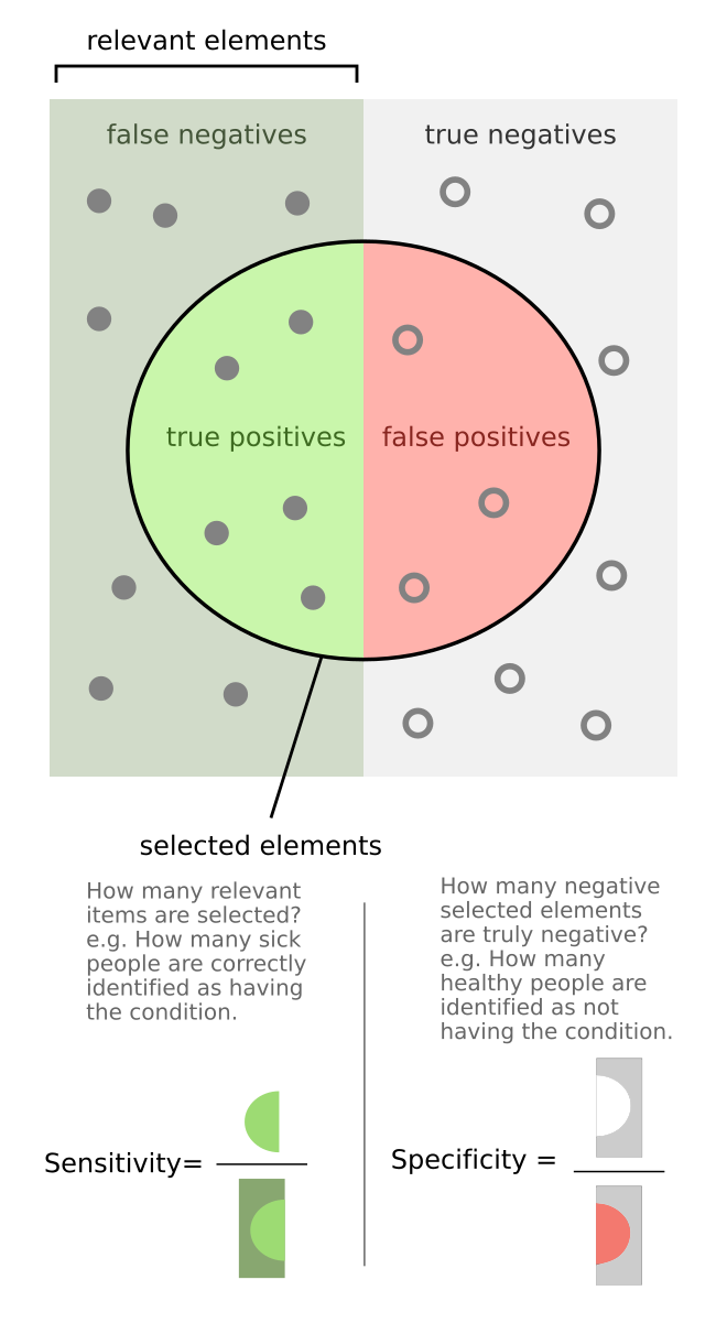
왼쪽: positive samples
오른쪽: negative smaples
원: positive라고 예측한 부분
일 때,
True positive: True라고 예측한 부분이 True가 맞음
False positive: True라고 예측한 부분이 False
True negative: False라고 예측한 부분이 True
False negative: False라고 예측한 부분이 False가 맞음

여기서 Sensitivity(민감도)란, $\frac{\text{True positive}}{\text{positive samples}}$
Specificity(특이도)란, $\frac{\text{False negative}}{\text{negative samples}}$

Distruibutions of Random Variables

확률 변수의 분포

• Probability density functions (PDFs, 확률 밀도 함수)
  

histogram일 때도 있고, continous한 모델일 수도 있음. 각각 Entry 값들 (Random variable)의 합이 1이고, 각각의 값들이 0~1 사이의 값을 가짐.

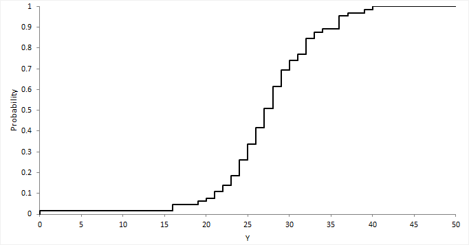
Probability/Cumulative Distributions

CDF(cumulative distribution function; 누적 분포 함수): PDF의 합을 구함

• $C(X \leq k) = \sum_{x\leq k} P(X=x)$
  

Descriptive Statistics

• Central tendency measures (중심 경향 측정)
  • mean(평균값): meaningful for symmetric distributions without outliers (특이점이 없는 대칭 분포에 의미가 있음) e.g., height and weight
  • median(중앙값): better for skewed distributions or data with outliers (skewness distributions(왜곡된 분포) 또는 노이즈가 많이 껴있는 곳에 더 좋음) e.g., wealth and income
• Variation or variability measures
  • variance(분산): square of the standard deviation(표준편차의 제곱)
    • $\hat{\sigma}=\sqrt{\frac{\sum_{i}^{n}(x_i-\bar{x})^2}{n-1}}$

Aggregation as Data Reduction

Representing a group of elements by a new derived element, like mean, min, count, sum reduces a large dataset to a small sumamry statistic
큰 데이터 셋 -> 작은 통계로 줄어듬

Such statistics can become features when taken over natural groups or clusters in the full data set
이러한 통계는 features로 연계될 수 있다.

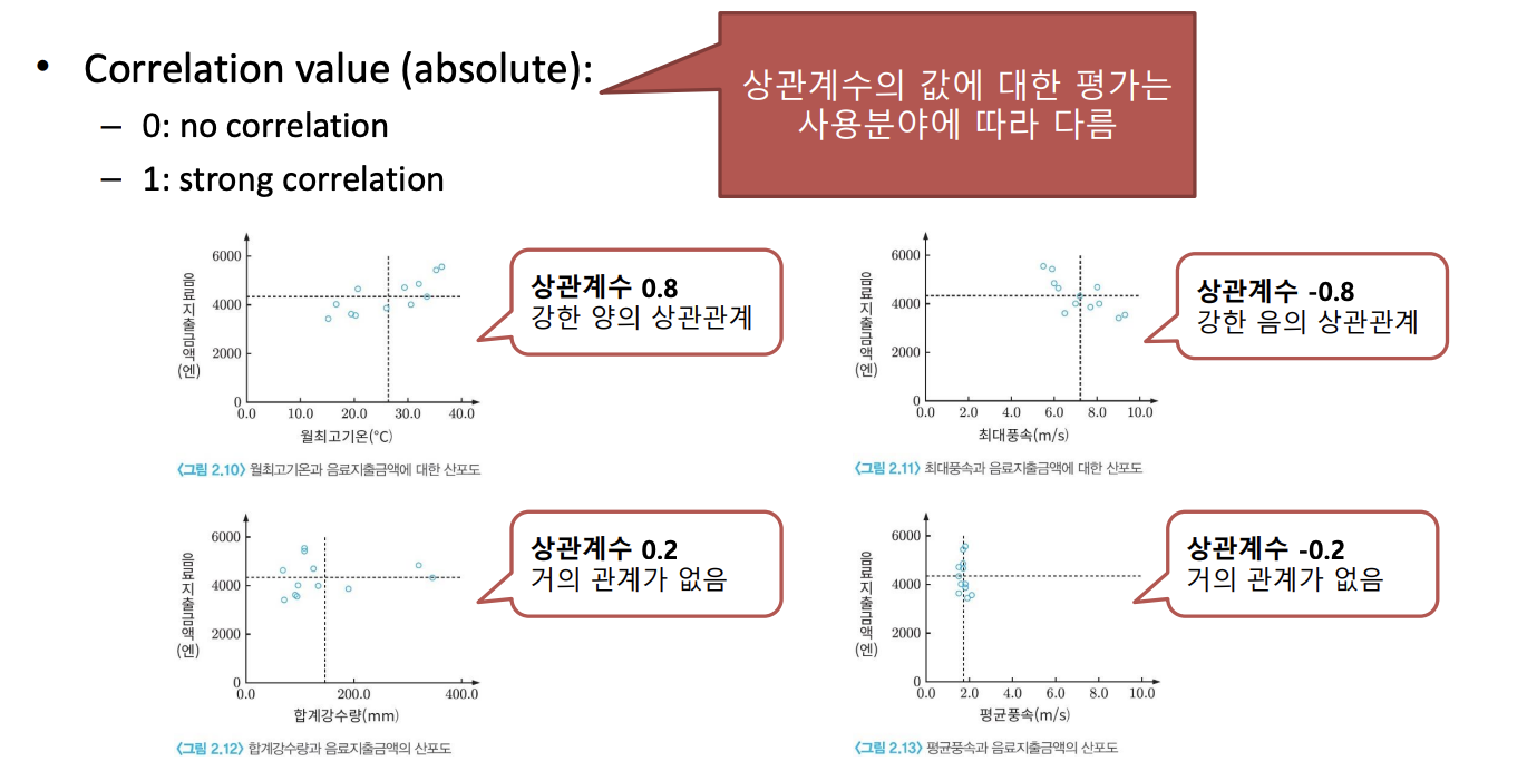
Correlation Analyses

Correlation 분석: 2개의 변수 간에 선형적인 관계를 파악하고 싶을 때 사용 (어느정도 관계가 있는 지)
Causal relationship(인과관계)를 나타내는 것은 아님! i.e., prediction model에 사용할 수 없음

Histogram

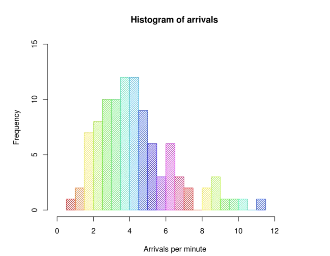Random vaiable을 만들 때 자주 사용됨

• “bin”: range of values (막대그래프의 폭)

• Quantization (이산화 과정)

• Effect of number of bins
  • Accurate assessment of distribution
    분포에 대한 정확성을 평가함
  • Computational complexity
    • kernel-based non-parametric PDF estimation (histogram or Parzen window)
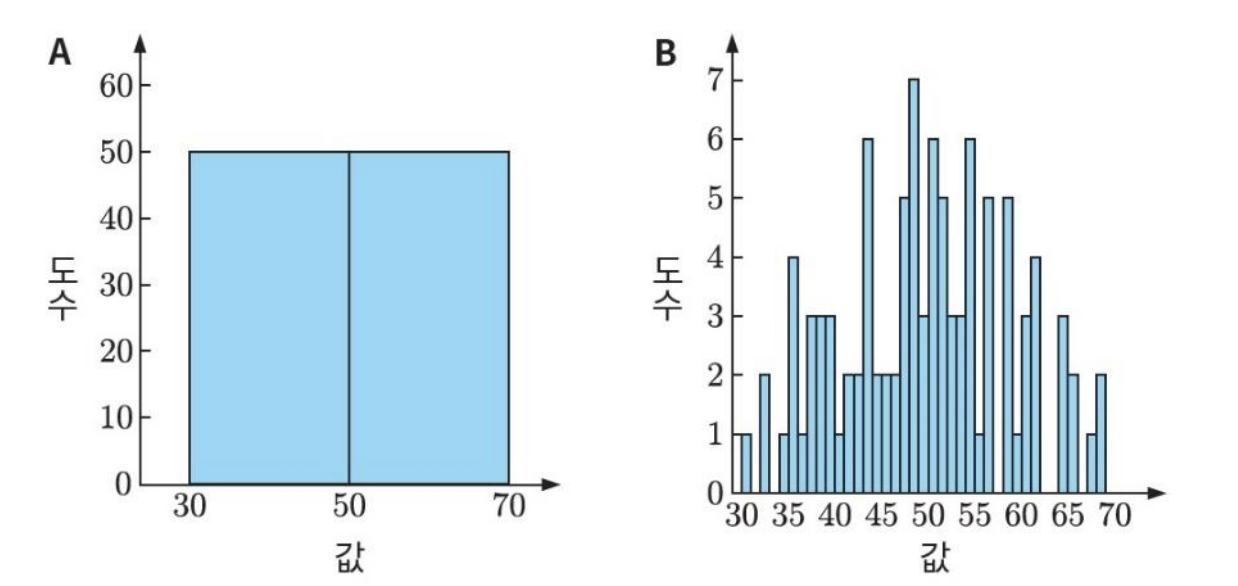
      분포를 표현하는 데에 영향을 끼침
      적당한 bin size를 찾는 것이 중요함

Historgram은 frequency (probabilistic distribution)을 의미하는 것이지 correlation을 의미하는 것이 아니다.

Correlation Coefficient (상관 계수)

• $Corr_{XY} = \frac{Var(XY)}{\sigma_X \sigma_Y}$
  • $Var(XY)$: covariance of X and Y (X와 Y의 공분산)
  • $\sigma_X$: standard deviation of X (X의 표준편차)
  • $\sigma_Y$: standard deviation of Y (Y의 표준편차)

Vector and Matrices

Vector

Vector: 값들의 1D array
Notation $x \in \mathbb{R}^n$ 대부분의 Vector는 아래와 같은 형태로 (세로로) 표현
\begin{align} x &= \begin{bmatrix} x_1 \newline x_2 \newline \vdots \newline x_n \end{bmatrix} \nonumber \end{align}

$x^T = [x_1, x_2, …, x_n]$, Transpose는 행과 열을 바꾸는 것이기 때문에 가로로 작성

Matrices

Matrix: 값들의 2D array Notation $A \in \mathbb{R}^{m\times n}$ \begin{align} A &= \begin{bmatrix} &A_{11} &\ldots &A_{1n} \newline &\vdots &\ddots &\vdots \newline &A_{m1} &\ldots &A_{mn} \end{bmatrix} \nonumber \end{align}

tabular data(table 형태로 표현되는 데이터)를 저장할 때 사용

Example

“Grade” table:

Person ID	HW1 Grade	HW2 Grade
5	100	80
6	60	80
100	100	100

이 데이터(primary key를 무시) Matrix로 표현하면

\begin{align} A \in \mathbb{R}^{3\times 2} = \begin{bmatrix} &100 &80 \newline &60 &80 \newline &100 &100 \end{bmatrix} \nonumber \end{align}

• Row major ordering: 100, 80, 60, 80, 100, 100
• Column major ordering: 100, 60, 100, 80, 80, 100

Higher dimensional matrices

“Higher dimensional matrices”는 Tensor라고 부른다.

Basic of linear algebra

아래 식을 vector matrix form으로 작성하면?

\begin{align} 4x_1-5x_2&=-13 \nonumber \newline -2x_1+3x_2&=9 \nonumber \end{align}

$Ax=b$ \begin{align} \text{where, } A= \begin{bmatrix} 4 &-5 \newline -2 &3 \end{bmatrix} , b = \begin{bmatrix} -13 \newline 9 \end{bmatrix}, \text{and } x = \begin{bmatrix}x_1 \newline x_2 \end{bmatrix} \nonumber \end{align}

Basic Matrix Operations

1. For $A, B \in \mathbb{R}^{m \times n}$, matrix addition/subtraction은 just the elementwise(각 요소 끼리만) addition/subtraction한다:
   • $C \in \mathbb{R}^{m \times n} = A+B \Leftrightarrow C_{ij} = A_{ij}+B_{ij}$
2. For $A \in \mathbb{R}^{m \times n}$, transpose is an operator that “flips” rows and columns (transpose는 행과 열을 뒤집음):
   • $C \in \mathbb{R}^{m \times n} = A^T \Leftrightarrow C_{ji} = A_{ij}$
3. For $A \in \mathbb{R}^{m \times n}, B \in \mathbb{R}^{n \times p}$ matrix multiplication(곱셈) is defined as
   • $C \in \mathbb{R}^{m \times p} = AB \Leftrightarrow C_{ij} = \sum_{k=1}^{n} A_{ik}B_{kj}$
4. Matrix multiplication is associative, distributive, but not commutative (size의 제약이 있기 때문)
   • $A(BC) = (AB)C \quad A(B+C)=AB+AC \quad (AB \neq BA)$

Matrix Inverse

Identity matrix: 대각 행렬만 다 1인 Matrix ($i==j?1:0lms$)
Identity matrix는 commutative하다.
Inverse matrix: 어떤 matrix에 Inverse matrix를 곱했을 때 Identity matrix가 나오는 Matrix
$A \in \mathbb{R}^{n \times n}, A^{-1} \in \mathbb{R}^{n \times n}$
$AA^{-1} = I = A^{-1}A$: commutative
이전에 나왔던 식 $Ax=b$를 inverse matrix를 사용해서 표연하면 간단하게 작성할 수 있다.
$x = A^{-1}b$

Some Miscellaneous Definitions/Properties

• Transpose of matrix multiplication (Matrix 곱의 transpose), $A\in \mathbb{R}^{m \times n}, B \in \mathbb{R}^{n \times p}$
  • $(AB)^T = B^TA^T$
• Inverse of product (Matrix 곱의 inverse), $A\in \mathbb{R}^{n \times n}, B \in \mathbb{R}^{n \times n}$
  • $(AB)^{-1}= B^{-1}A^{-1}$
• Inverse of product (Matrix 곱의 inverse), $A\in \mathbb{R}^{n \times n}, B \in \mathbb{R}^{n \times n}$
  • $(AB)^{-1}= B^{-1}A^{-1}$
• Inner product: for $x, y \in \mathbb{R}^n$
  • $x^Ty \in \mathbb{R} = \sum^{n}_{i=1}x_iy_i$
• Vector norms: for $x \in \mathbb{R}^n$, we use $||x||_2$ to denote Euclidean norm
  • $||x||_2 = (x^Tx)^{\frac{1}{2}}$

Norm? Size of Vector

• $L_1$ Norm ($L_2$ Norm과 함께 주로 사용): 절대값의 합
  • $||x||_1 = \sum|x_i|$
• $L_2$ Norm (일반적으로 사용): 제곱의 합을 sqrt
  • $||x||_2 = \sqrt{\sum x^2_i} = (x^Tx)^{\frac{1}{2}}$
• $L_p$ Norm
  • $||x||_p = \sqrt[p]{\sum|x_i|^p}$
• $L_\infty$ Norm
  • $||x||_\infty = max(|x_1|, |x2|, …, |x_n|) = \sup_i|x_i|$

Brief vector calculus

Vector Derivative

Vector by scalar

(Vector를 scalar로 미분): 모든 원소를 스칼라로 미분
$y = [y1, y2, …, y_m]^T$일 때
\begin{align} \frac{\partial y}{\partial x} &= \begin{bmatrix} \frac{\partial y_1}{\partial x} \newline \frac{\partial y_2}{\partial x} \newline \vdots \newline \frac{\partial y_m}{\partial x} \end{bmatrix} \nonumber \end{align}

Scalar to Vector

(Scalar를 Vector로 미분): 벡터 각각에 편미분 = gradient라고 함 $x = [x1, x2, …, x_n]^T$일 때
$\frac{\partial y}{\partial x} = [\frac{\partial y}{\partial x_1}, \frac{\partial y}{\partial x_2}, …, \frac{\partial y}{\partial x_n}]$ \begin{align} \nabla f &= \begin{bmatrix} \frac{\partial f}{\partial x_1} \newline \frac{\partial f}{\partial x_2} \newline \vdots \newline \frac{\partial f}{\partial x_n} \end{bmatrix} \nonumber = (\frac{\partial f}{\partial x})^T \end{align}

Vector to Vector

(Vector를 Vector로 미분): 각각의 원소끼리 미분 => Matrix가 된다! (Jacobian matrix) $x = [x1, x2, …, x_n]^T, y = [y1, y2, …, y_m]^T$일 때
$\frac{\partial y}{\partial x} = [\frac{\partial y}{\partial x_1}, \frac{\partial y}{\partial x_2}, …, \frac{\partial y}{\partial x_n}]$ \begin{align} \frac{\partial y}{\partial x} = \begin{bmatrix} \frac{\partial y_1}{\partial x_1} &\frac{\partial y_1}{\partial x_2} &\ldots &\frac{\partial y_1}{\partial x_n} \newline \frac{\partial y_2}{\partial x_1} &\frac{\partial y_2}{\partial x_2} &\ldots &\frac{\partial y_2}{\partial x_n} \newline \vdots &\vdots &\ddots &\vdots \newline \frac{\partial y_m}{\partial x_1} &\frac{\partial y_m}{\partial x_2} &\ldots &\frac{\partial y_m}{\partial x_n} \end{bmatrix} \nonumber \end{align}

Vector Calculus (Derivatives): PCA

Principal component analysis (PCA, 주성분 분석) 데이터의 차원을 축소 시켰을 때 정보량의 손실이 가장 적은 방향(Vector)을 찾고 싶다

$X = {(x_i, y_i, z_i)^T | i=1, …, n}$

• 각각의 Data point는 3D-vector라고 생각함
• n: 요소의 개수
• $x_i, y_i, z_i$: 각각의 i번째 포인트의 값

$u = \frac{1}{n}\sum^n_{i=1}X_i$

• mean vector

$C = \frac{1}{n}\sum^{n}_{i=1} X_iX_i^T - uu^T$

• Covariance matrix